Best Practices For Data Annotation

Here we take a closer look at some experimental scenarios that every scientist might face on a more or less regular basis. With these examples, we aim to provide you with the best practices for data annotation in isa.study.xlsx and isa.assay.xlsx files allowing you to generate machine-readable and thereby, interoperable and reproducible data. Do not hesitate to contact us if you think that we are missing some urgent examples or if you have any further questions.

Annotation of time series experiments

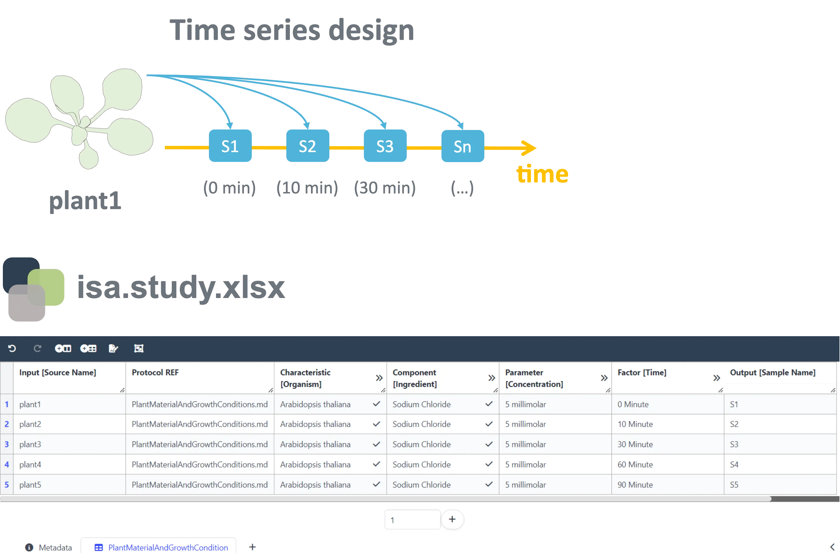
As an example, we will walk you through a simple ARC and discuss good practices for annotation along the way. In our first scenario we take a look at the annotation of time course patterns. Let’s imagine a study in which our plant of interest (plant1), Arabidopsis thaliana (Characteristic [Organism]), was exposed to salt stress (Component [Ingredient]) for a given time. To investigate the cellular response, you harvested samples at various time points after exposure to the stressor: S1 is harvested right away, S2 after 10 minutes, and so on. This information was stored within the isa.study.xlsx file.

You should use the Factor building block in such a case to annotate the time after exposure and thereby the sampling point in the isa.study.xlsx file, as this time period will ultimately result in the given output, when all remaining parameters for treatment and analysis were identical.

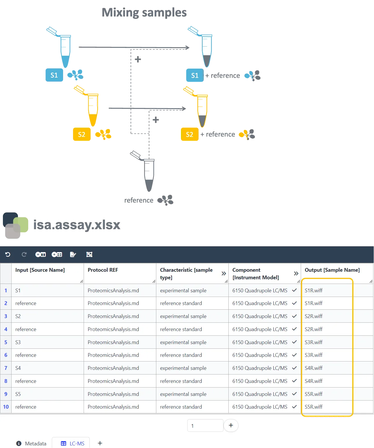
Annotation of mixed samples

This example can be of relevance when you are carrying out labeling experiments or when you are spiking your samples with an internal standard for absolute quantification. The isa.assay.xlsx file below displays the best practice for annotating the mixing of experimental samples with a reference prior to LC/MS analysis (Component [Instrumentation]). By listing every data file twice, it becomes clear that the analyzed files originated from the combination of an experimental sample and a reference, e.g. spiking of S1 with the reference resulted in the output file name S1R.wiff.

Annotation of biological/technical replicates and sub-processes

In the following scenario we focus on annotating the origin and relationship between biological/technical replicates and managing sub-processes within an assay. We start with the five samples (S1, S2, …, S5), originating from the isa.study.xlsx file. We want to perform a transcriptomics analysis but before that we have to extract RNA from our samples. Some processes and lab procedures cannot be described coherently in one isa table, even though they are part of the same assay. In such case, you can split subprocesses into different sheets of the same isa table. For example, here the extraction of RNA is described in the first sheet with an output being the RNA samples (rna_sample1, …). Then on the next sheet is the table representing the sequencing itself. As you can see, the input becomes the output from the previous sheet, thus, indicating the processes are sequential. In the same manner, samples and processes are being connected across studies and assays within an ARC. While performing the RNA sequencing, three technical replicates per sample are generated (Characteristic [technical replicate]). However, each replicate results in its own data file.

Connecting inputs and outputs

A key objective of the ARC is to trace each finding or result back to its specific biological experiment. Achieving this requires linking dataset files to their corresponding individual samples. To accomplish this, we follow a sequence of processes with defined inputs and outputs. Certain inputs and outputs may need to be reused or reproduced, while some processes may need to be applied to different inputs.